CT Reconstruction

Project Repository : https://github.com/jihoojung0106/cbct_recon

1. Introduction

In dental CT, the primary focus is reconstructing 3D images of objects captured using projection data sets. The objective of this project is to implement the FDK algorithm, one of the fundamental algorithms in CT data reconstruction, on CPU. To achieve this, we present two models: a simplified model implemented using MATLAB and a formal model implemented using C.

2. Background Study

2.1 Back Projection

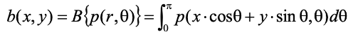
Let’s first examine the most fundamental technique, Back Projection. Considering \(p_{\theta}(r)\) as the projection at angle θ, we can obtain the sinogram \(p(r,\theta)\) by performing the Radon Transform using the following equation.

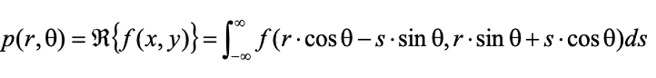
Using the integral expression below, summing up all the Sinogram values for every angle yields the reconstructed image.

2.2 Filtered Back Projection

The simplest back projection method suffers from blurring artifacts in the reconstructed image. However, the Filtered Back Projection algorithm overcomes this drawback. The Filtered Back Projection (FBP) technique involves filtering the sinogram before performing back projection.

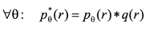
Let \(q(r)\) represent the filter function. The filtering process is described by the following equation. High-pass filters are employed to counteract the smoothing effect induced by back projection and to restore high-frequency components.

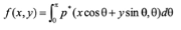
By backprojecting the filtered data as described in the equation below, a reconstructed image can be generated.

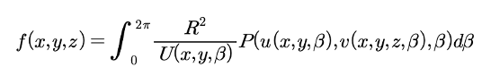
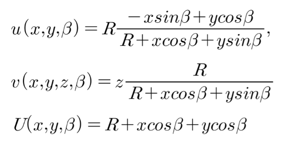
2.3 FDK

The FDK algorithm, proposed by Feldkamp, Davis, and Kress, is an enhancement of the FBP algorithm specifically designed for cone beam CT applications.

3. Model

3.1 Dataset

• Input : projection data
  • 1) Type: 706 .RAW files, 16bit unsigned
  • 2) Width and Height: 1628 pixel,1500 pixel
  • 3) Pitch: 0.098 mm
• Output : reconstructed image data
  • 1) Type: 450 .RAW files, 16bit signed
  • 2) Volume size x,y,z: 750 pixel, 750 pixel,450 pixel
  • 3) Volume pitch: 0.20 mm
  • 4) Volume offset z: 45 pixel

3.2 Processing Steps

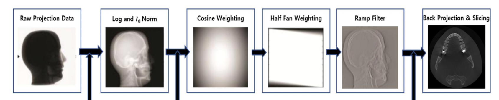
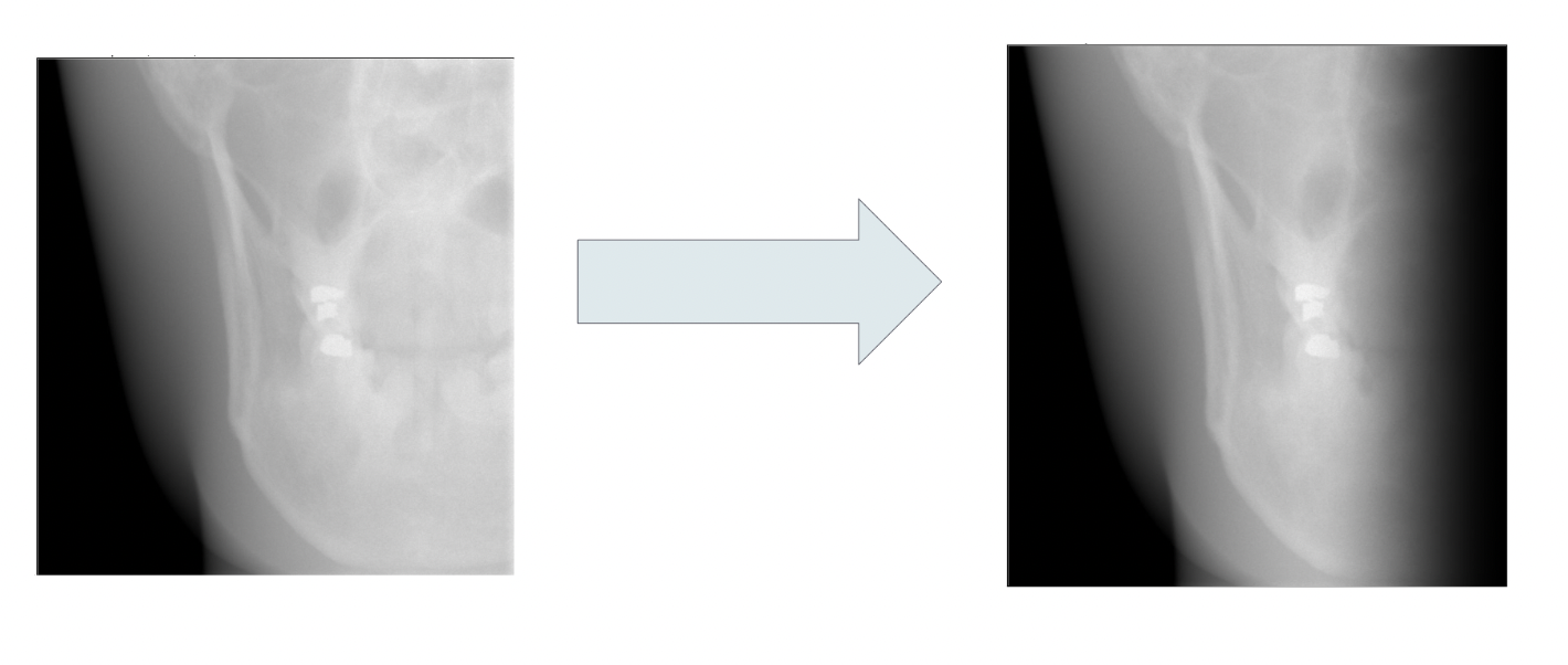
1) Log Transform and Normalization

The raw projection data is converted into a sinogram using the integral expression discussed earlier.

2) Cosine Weighting and Half-fan Weighting

• Cosine Weighting : By applying cosine weighting, varying weights are multiplied to each projection based on the angle and spatial frequency, compensating for the non-uniform distribution of projections.
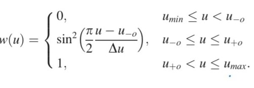
• Half-fan Weighting : Half-fan weighting is employed to compensate for the half-fan geometry, where the detector is skewed towards one side of the object. This is done according to the following equation.

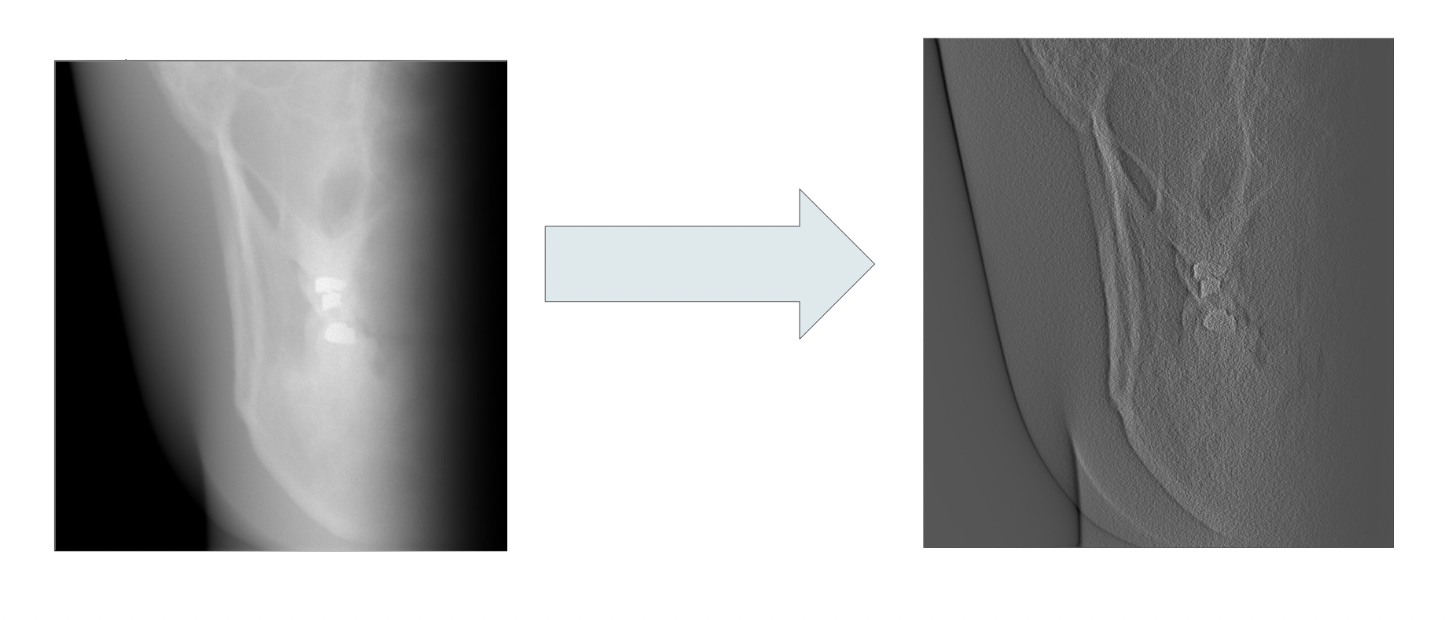
3) High Pass Filtering

The process entails applying Fourier transform, followed by the application of a ramp filter, and concluding with application of inverse Fourier transform.

4) Backprojection

Backprojection is performed using the point-driven method.

5) HU scaling

By utilizing the voxel values from the reconstructed volume along with their corresponding Hounsfield Units (HU), a linear conversion is executed to scale the values based on the voxel information. Subsequently, the values undergo a conversion from floating-point to integer.

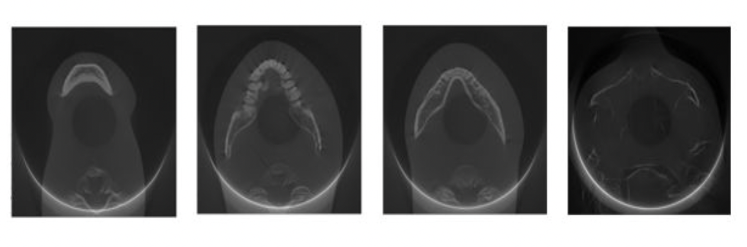
4. Results

Reconstruction slices (from left to right: 1st, 200th, 300th, 400th).

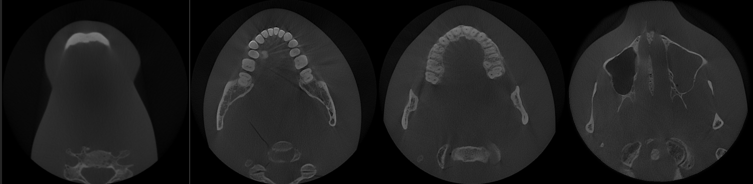
Reference output (from left to right: 1st, 200th, 300th, 400th).